(1). nuclear norm:
∣ ∣ X ∣ ∣ ∗ = ∣ ∣ singular values ∣ ∣ 1 ||X||_* = ||\text{singular values}||_1 ∣ ∣ X ∣ ∣ ∗ = ∣ ∣ singular values ∣ ∣ 1
(2). frobenius norm:
∣ ∣ X ∣ ∣ F = ∑ i , j X i , j 2 = ∣ ∣ singular values ∣ ∣ 2 ||X||_F =\sqrt{\sum_{i,j}X_{i,j}^2} = ||\text{singular values}||_2 ∣ ∣ X ∣ ∣ F = ∑ i , j X i , j 2 = ∣ ∣ singular values ∣ ∣ 2
∣ ∣ X ∣ ∣ F 2 = ∑ i , j X i , j 2 = t r ( X T X ) = t r ( V Λ U T U Λ V T ) = t r ( V Λ 2 V T ) = t r ( Λ 2 V T V ) = t r ( Λ 2 ) ||X||_F^2 = \sum_{i,j}X_{i,j}^2 \\
~~~~~~~~~~~~~~~= tr(X^TX) \\
~~~~~~~~~~~~~~~~~~~~~~~~~~~~= tr(V \Lambda U^T U \Lambda V^T) \\
~~~~~~~~~~~~~~~~~~= tr(V \Lambda^2V^T) \\
~~~~~~~~~~~~~~~~~~= tr(\Lambda^2 V^TV) \\
~~~~~~~~ = tr(\Lambda^2) ∣ ∣ X ∣ ∣ F 2 = i , j ∑ X i , j 2 = t r ( X T X ) = t r ( V Λ U T U Λ V T ) = t r ( V Λ 2 V T ) = t r ( Λ 2 V T V ) = t r ( Λ 2 ) (3). spectral norm:
∣ ∣ X ∣ ∣ 2 = s u p v ∣ ∣ X v ∣ ∣ 2 ∣ ∣ v ∣ ∣ 2 = ∣ ∣ singular values ∣ ∣ i n f ||X||_2 = sup_v{ \frac{||Xv||_2}{||v||_2}}=|| \text{singular values}||_{inf} ∣ ∣ X ∣ ∣ 2 = s u p v ∣ ∣ v ∣ ∣ 2 ∣ ∣ X v ∣ ∣ 2 = ∣ ∣ singular values ∣ ∣ i n f
(1-norm and inf-norm are a pair of dual norms.)
min . Z , E rank ( Z ) + λ ∣ ∣ E ∣ ∣ 2 , 1 \text{min}._{Z,E} ~~\text{rank}(Z) + \lambda ||E||_{2,1} min . Z , E rank ( Z ) + λ ∣ ∣ E ∣ ∣ 2 , 1 s.t. X = A Z + E \text{s.t.} ~~~~X = AZ + E s.t. X = A Z + E (∣ ∣ E ∣ ∣ 2 , 1 ||E||_{2,1} ∣ ∣ E ∣ ∣ 2 , 1
Z ∈ R d ∗ n Z \in \mathbb{R}^{d*n} Z ∈ R d ∗ n X ∈ R 1000 ∗ 50 X \in \mathbb{R}^{1000*50} X ∈ R 1 0 0 0 ∗ 5 0
In the face example, since there are only 5 people in
50 images, the "rank" of the data matrix is 5, so we
want to transform the data matrix to low-rank
representation.
Suppose A A A Z Z Z X X X A Z + E AZ+E A Z + E E E E
Since minimizing the rank of Z Z Z r a n k ( Z ) rank(Z) r a n k ( Z ) ∣ ∣ X ∣ ∣ ∗ ||X||_* ∣ ∣ X ∣ ∣ ∗ ∣ ∣ X ∣ ∣ ∗ = ∣ ∣ singular values ∣ ∣ 1 ||X||_* = ||\text{singular values}||_1 ∣ ∣ X ∣ ∣ ∗ = ∣ ∣ singular values ∣ ∣ 1
min . Z , E ∣ ∣ Z ∣ ∣ ∗ + λ ∣ ∣ E ∣ ∣ 2 , 1 \text{min}._{Z,E} ~~||Z||_* + \lambda ||E||_{2,1} min . Z , E ∣ ∣ Z ∣ ∣ ∗ + λ ∣ ∣ E ∣ ∣ 2 , 1 s.t. X = A Z + E \text{s.t.} ~~~~X = AZ + E s.t. X = A Z + E Consider the regularized frobenius norm minimization
problem
min x . f ( x ) = 1 2 ∣ ∣ X − Y ∣ ∣ F 2 + τ ∣ ∣ X ∣ ∣ ∗ \text{min}_x.~~ f(x) = \frac{1}{2}||X-Y||_F^2 + \tau ||X||_* min x . f ( x ) = 2 1 ∣ ∣ X − Y ∣ ∣ F 2 + τ ∣ ∣ X ∣ ∣ ∗ ∂ f ∂ x = X − Y + τ ∂ ∣ ∣ X ∣ ∣ ∗ \frac{\partial f}{\partial x} = X - Y + \tau \partial||X||_* ∂ x ∂ f = X − Y + τ ∂ ∣ ∣ X ∣ ∣ ∗ f ( x ) f(x) f ( x ) 0 ⃗ ∈ ∂ f ∂ x \vec{0} \in \frac{\partial f}{\partial x} 0 ∈ ∂ x ∂ f f f f ∂ f ∂ x \frac{\partial f}{\partial x} ∂ x ∂ f f f f
We apply singular value decomposition to Y Y Y
Y = U Σ V T = U 0 Σ 0 V 0 T + U 1 Σ 1 V 1 T Y = U \Sigma V^T \\
~~~~~~~~~~~~~~~~~~~~~~= U_0 \Sigma_0 V_0^T + U_1 \Sigma_1 V_1^T Y = U Σ V T = U 0 Σ 0 V 0 T + U 1 Σ 1 V 1 T where d i a g ( Σ 0 ) > τ diag(\Sigma_0)>\tau d i a g ( Σ 0 ) > τ d i a g ( Σ 0 ) < = τ diag(\Sigma_0)<=\tau d i a g ( Σ 0 ) < = τ
Define singular value shrink operator as
D τ ( Σ ) = diag ( { σ i − τ } + ) = diag ( max { σ i − τ , 0 } ) D_{\tau}(\Sigma) = \text{diag}(\{\sigma_i - \tau\}_+)
= \text{diag}( \text{max}\{\sigma_i - \tau, 0\}) D τ ( Σ ) = diag ( { σ i − τ } + ) = diag ( max { σ i − τ , 0 } ) D τ ( X ) = U D τ ( Σ ) V T ( X = U Σ V T is the SVD of X) D_{\tau}(X) = U D_{\tau}(\Sigma)V^T
~~~~~~\text{($X = U \Sigma V^T$ is the SVD of X)} D τ ( X ) = U D τ ( Σ ) V T ( X = U Σ V T is the SVD of X) Perform singular value shrinkage on Y Y Y
D τ ( Y ) = D τ ( U 0 Σ 0 V 0 T + U 1 Σ 1 V 1 T ) = U 0 ( Σ 0 − τ I ) V 0 T D_{\tau}(Y) ~~~= D_{\tau}(U_0 \Sigma_0 V_0^T + U_1 \Sigma_1 V_1^T) \\
= U_0 (\Sigma_0 - \tau I)V_0^T D τ ( Y ) = D τ ( U 0 Σ 0 V 0 T + U 1 Σ 1 V 1 T ) = U 0 ( Σ 0 − τ I ) V 0 T Y − D τ ( Y ) = τ ( U 0 V 0 T + 1 τ U 1 Σ 1 V 1 T ) Y - D_{\tau}(Y) = \tau(U_0V_0^T + \frac{1}{\tau}U_1 \Sigma_1 V_1^T) Y − D τ ( Y ) = τ ( U 0 V 0 T + τ 1 U 1 Σ 1 V 1 T ) The subgradient of nuclear norm is defined by
∂ ∣ ∣ X ∣ ∣ ∗ = { U V T + W ∣ U T W = 0 , W V = 0 , ∣ ∣ W ∣ ∣ 2 < = 1 } \partial ||X||_* = \{UV^T + W| U^TW=0, WV=0, ||W||_2<=1\} ∂ ∣ ∣ X ∣ ∣ ∗ = { U V T + W ∣ U T W = 0 , W V = 0 , ∣ ∣ W ∣ ∣ 2 < = 1 } Let U = U 0 , V = V 0 , W = 1 τ U 1 Σ 1 V 1 T U = U_0, V = V_0, W = \frac{1}{\tau}U_1 \Sigma_1 V_1^T U = U 0 , V = V 0 , W = τ 1 U 1 Σ 1 V 1 T Y − D τ ( Y ) ∈ τ ∂ ∣ ∣ X ∣ ∣ ∗ Y-D_{\tau}(Y) \in \tau \partial ||X||_* Y − D τ ( Y ) ∈ τ ∂ ∣ ∣ X ∣ ∣ ∗
Let X = D τ ( Y ) X = D_{\tau}(Y) X = D τ ( Y ) X − Y + Y − D τ ( Y ) = 0 ∈ ∂ f ∂ x X - Y + Y - D_{\tau}(Y) =0 \in \frac{\partial f}{\partial x} X − Y + Y − D τ ( Y ) = 0 ∈ ∂ x ∂ f X = D τ ( Y ) X = D_{\tau}(Y) X = D τ ( Y ) 1 2 ∣ ∣ X − Y ∣ ∣ F 2 + τ ∣ ∣ X ∣ ∣ ∗ \frac{1}{2}||X-Y||_F^2 + \tau ||X||_* 2 1 ∣ ∣ X − Y ∣ ∣ F 2 + τ ∣ ∣ X ∣ ∣ ∗
min . f ( x ) s.t. h i ( x ) = 0 \text{min}. ~~~~~~f(x) \\
\text{s.t.} ~~h_i(x)=0 min . f ( x ) s.t. h i ( x ) = 0 L ( x , v ) = f ( x ) + ∑ i v i h i ( x ) L(x,v) = f(x) + \sum_i v_i h_i(x) L ( x , v ) = f ( x ) + i ∑ v i h i ( x ) Define the augmented lagrangian as
A ( x , v , c ) = L ( x , v ) + c 2 ∣ ∣ h i ( x ) ∣ ∣ 2 2 A(x,v,c) = L(x,v) + \frac{c}{2} ||h_i(x)||_2^2 A ( x , v , c ) = L ( x , v ) + 2 c ∣ ∣ h i ( x ) ∣ ∣ 2 2 The optimality condition for the original problem is
1.h i ( x ∗ ) = 0 h_i(x^*) = 0 h i ( x ∗ ) = 0
2.∇ x L ( x ∗ , v ∗ ) = ∇ f ( x ∗ ) + ∑ i v i ∇ h i ( x ∗ ) = 0 \nabla_xL(x^*, v^*) = \nabla f(x^*) + \sum_i v_i \nabla h_i(x^*) = 0 ∇ x L ( x ∗ , v ∗ ) = ∇ f ( x ∗ ) + ∑ i v i ∇ h i ( x ∗ ) = 0
if x ∗ , v ∗ x^*, v^* x ∗ , v ∗
∇ x A ( x ∗ , v ∗ , c ) = ∇ L x ( x ∗ , v ∗ ) + c ∑ i h i ( x ∗ ) ∇ h i ( x ∗ ) = 0 \nabla_x A(x^*,v^*,c) = \nabla L_x(x^*,v^*) + c \sum_i h_i(x^*) \nabla h_i(x^*) = 0 ∇ x A ( x ∗ , v ∗ , c ) = ∇ L x ( x ∗ , v ∗ ) + c i ∑ h i ( x ∗ ) ∇ h i ( x ∗ ) = 0 x ∗ , v ∗ x^*, v^* x ∗ , v ∗
When we solve the original problem with augmented
lagangian, we want to minimize the augmented lagrangian
and keep ∇ x A ( x , v , c ) = ∇ x L ( x , v ) \nabla_xA(x,v,c) = \nabla_xL(x,v) ∇ x A ( x , v , c ) = ∇ x L ( x , v )
x ′ = a r g m i n x A ( x , v , c ) x' = argmin_x A(x,v,c) x ′ = a r g m i n x A ( x , v , c ) ∇ x A ( x ′ , v , c ) = ∇ f ( x ′ ) + ∑ i v i ∇ h i ( x ) + c ∑ i h i ( x ∗ ) ∇ h i ( x ∗ ) \nabla_x A(x',v,c) = \nabla f(x') + \sum_i v_i \nabla h_i(x) + c \sum_i h_i(x^*) \nabla h_i(x^*) ∇ x A ( x ′ , v , c ) = ∇ f ( x ′ ) + i ∑ v i ∇ h i ( x ) + c i ∑ h i ( x ∗ ) ∇ h i ( x ∗ ) ∇ L ( x ′ , v ′ ) = ∇ f ( x ′ ) + ∑ i v i ′ ∇ h i ( x ′ ) \nabla L(x',v') = \nabla f(x') + \sum_i v_i' \nabla h_i(x') ∇ L ( x ′ , v ′ ) = ∇ f ( x ′ ) + i ∑ v i ′ ∇ h i ( x ′ ) To keep ∇ x A ( x ′ , v , c ) = ∇ L ( x ′ , v ′ ) \nabla_x A(x',v,c) = \nabla L(x',v') ∇ x A ( x ′ , v , c ) = ∇ L ( x ′ , v ′ ) v i ′ = v i + c ∗ h i ( x ′ ) v_i' = v_i + c*h_i(x') v i ′ = v i + c ∗ h i ( x ′ )
The augmented lagrangian algorithm
repeat until convergence{
    x' = argmin_x L(x,v)
    v_i' = v_i + c * h_i(x')
    x = x'
    v = v'
}
The low-rank representation problem
min Z , E ∣ ∣ Z ∣ ∣ ∗ + λ ∣ ∣ E ∣ ∣ 2 , 1 \text {min}_{Z,E} ~~||Z||_* + \lambda ||E||_{2,1} min Z , E ∣ ∣ Z ∣ ∣ ∗ + λ ∣ ∣ E ∣ ∣ 2 , 1 s.t. X = A Z + E \text {s.t.} ~~~X = AZ + E s.t. X = A Z + E Transform is to the equivalent problem
min Z , E ∣ ∣ J ∣ ∣ ∗ + λ ∣ ∣ E ∣ ∣ 2 , 1 \text {min}_{Z,E} ~~||J||_* + \lambda ||E||_{2,1} min Z , E ∣ ∣ J ∣ ∣ ∗ + λ ∣ ∣ E ∣ ∣ 2 , 1 s.t. X = A Z + E \text {s.t.} ~~~X = AZ + E s.t. X = A Z + E Form the lagrangian and the augmented lagrangian
L ( Z , E , J , Y 1 , Y 2 ) = ∣ ∣ J ∣ ∣ ∗ + λ ∣ ∣ E ∣ ∣ 2 , 1 + t r ( Y 1 T ( X − A Z − E ) ) + t r ( Y 2 T ( Z − J ) ) L(Z,E,J,Y_1,Y_2) = ||J||_* + \lambda ||E||_{2,1} +
tr(Y_1^T(X-AZ-E)) + tr(Y_2^T(Z-J)) L ( Z , E , J , Y 1 , Y 2 ) = ∣ ∣ J ∣ ∣ ∗ + λ ∣ ∣ E ∣ ∣ 2 , 1 + t r ( Y 1 T ( X − A Z − E ) ) + t r ( Y 2 T ( Z − J ) ) A ( Z , E , J , Y 1 , Y 2 , c ) = ∣ ∣ J ∣ ∣ ∗ + λ ∣ ∣ E ∣ ∣ 2 , 1 + t r ( Y 1 T ( X − A Z − E ) ) + t r ( Y 2 T ( Z − J ) ) + c 2 ∣ ∣ X − A Z − E ∣ ∣ F 2 + c 2 ∣ ∣ Z − J ∣ ∣ F 2 A(Z,E,J,Y_1,Y_2, c) = ||J||_* + \lambda ||E||_{2,1} +
tr(Y_1^T(X-AZ-E)) + tr(Y_2^T(Z-J)) +
\frac{c}{2} ||X-AZ-E||_F^2 + \frac{c}{2} ||Z-J||_F^2 A ( Z , E , J , Y 1 , Y 2 , c ) = ∣ ∣ J ∣ ∣ ∗ + λ ∣ ∣ E ∣ ∣ 2 , 1 + t r ( Y 1 T ( X − A Z − E ) ) + t r ( Y 2 T ( Z − J ) ) + 2 c ∣ ∣ X − A Z − E ∣ ∣ F 2 + 2 c ∣ ∣ Z − J ∣ ∣ F 2
Update J J J
∇ J A ( Z , E , J , Y 1 , Y 2 , c ) = c ∗ [ J − Z ] − Y 2 + ∂ ∣ ∣ J ∣ ∣ ∗ \nabla_JA(Z,E,J,Y_1,Y_2,c) = c * [J - Z] - Y_2 + \partial ||J||_* ∇ J A ( Z , E , J , Y 1 , Y 2 , c ) = c ∗ [ J − Z ] − Y 2 + ∂ ∣ ∣ J ∣ ∣ ∗ = c [ J − ( Z + 1 c Y 2 ) ] + ∂ ∣ ∣ J ∣ ∣ ∗ = 0 = c[J-(Z+\frac{1}{c}Y_2)] + \partial ||J||_*
=0 = c [ J − ( Z + c 1 Y 2 ) ] + ∂ ∣ ∣ J ∣ ∣ ∗ = 0 [ J − ( Z + 1 c Y 2 ) ] + 1 c ∂ ∣ ∣ J ∣ ∣ ∗ = 0 [J-(Z+\frac{1}{c}Y_2)] + \frac{1}{c}\partial ||J||_*=0 [ J − ( Z + c 1 Y 2 ) ] + c 1 ∂ ∣ ∣ J ∣ ∣ ∗ = 0 Apply SVD on Z + 1 c Y 2 Z + \frac{1}{c}Y_2 Z + c 1 Y 2
Z + 1 c Y 2 = U 0 Σ 0 V 0 T + U 1 Σ 1 V 1 T Z + \frac{1}{c}Y_2 = U_0 \Sigma_0V_0^T +
U_1 \Sigma_1V_1^T Z + c 1 Y 2 = U 0 Σ 0 V 0 T + U 1 Σ 1 V 1 T where d i a g ( Σ 0 ) > 1 / c diag(\Sigma_0) > 1/c d i a g ( Σ 0 ) > 1 / c d i a g ( Σ 1 ) < = 1 / c diag(\Sigma_1) <= 1/c d i a g ( Σ 1 ) < = 1 / c
Perform singular value shrinkage with threshold
1 / c 1/c 1 / c Z + 1 c Y 2 Z + \frac{1}{c}Y_2 Z + c 1 Y 2
D 1 / c ( Z + 1 c Y 2 ) = U 0 ( Σ 0 − 1 c I ) V 0 T D_{1/c}(Z + \frac{1}{c}Y_2) = U_0(\Sigma_0- \frac{1}{c}I) V_0^T D 1 / c ( Z + c 1 Y 2 ) = U 0 ( Σ 0 − c 1 I ) V 0 T ( Z + 1 c Y 2 ) − D 1 / c ( Z + 1 c Y 2 ) = U 1 Σ 1 V 1 T + 1 c U 0 V 0 T (Z + \frac{1}{c}Y_2) - D_{1/c}(Z + \frac{1}{c}Y_2) =
U_1 \Sigma_1V_1^T + \frac{1}{c}U_0V_0^T ( Z + c 1 Y 2 ) − D 1 / c ( Z + c 1 Y 2 ) = U 1 Σ 1 V 1 T + c 1 U 0 V 0 T = 1 c ( U 0 V 0 T + c ∗ U 1 Σ 1 V 1 T ) = \frac{1}{c} (U_0V_0^T + c * U_1 \Sigma_1V_1^T) = c 1 ( U 0 V 0 T + c ∗ U 1 Σ 1 V 1 T ) Since ∂ ∣ ∣ X ∣ ∣ ∗ = { U V T + W ∣ U T W = 0 , W V = 0 , ∣ ∣ W ∣ ∣ 2 < = 1 } \partial ||X||_* = \{UV^T + W | U^TW=0, WV=0, ||W||_2<=1\} ∂ ∣ ∣ X ∣ ∣ ∗ = { U V T + W ∣ U T W = 0 , W V = 0 , ∣ ∣ W ∣ ∣ 2 < = 1 } U = U 0 , V = V 0 , W = c ∗ U 1 Σ 1 V 1 T U=U_0, V=V_0, W=c * U_1 \Sigma_1V_1^T U = U 0 , V = V 0 , W = c ∗ U 1 Σ 1 V 1 T
1 c ( U 0 V 0 T + c ∗ U 1 Σ 1 V 1 T ) = ( Z + 1 c Y 2 ) − D 1 / c ( Z + 1 c Y 2 ) ∈ 1 c ∂ ∣ ∣ J ∣ ∣ ∗ \frac{1}{c} (U_0V_0^T + c * U_1 \Sigma_1V_1^T) =
(Z + \frac{1}{c}Y_2) - D_{1/c}(Z + \frac{1}{c}Y_2)
\in \frac{1}{c} \partial||J||_* c 1 ( U 0 V 0 T + c ∗ U 1 Σ 1 V 1 T ) = ( Z + c 1 Y 2 ) − D 1 / c ( Z + c 1 Y 2 ) ∈ c 1 ∂ ∣ ∣ J ∣ ∣ ∗ J ∗ = ( Z + 1 c Y 2 ) − 1 c ∂ ∣ ∣ J ∣ ∣ ∗ = D 1 / c ( Z + 1 c Y 2 ) J^* = (Z + \frac{1}{c}Y_2) - \frac{1}{c} \partial||J||_* = D_{1/c}(Z + \frac{1}{c}Y_2) J ∗ = ( Z + c 1 Y 2 ) − c 1 ∂ ∣ ∣ J ∣ ∣ ∗ = D 1 / c ( Z + c 1 Y 2 )
Update Z Z Z
∇ Z A ( Z , E , J , Y 1 , Y 2 , c ) = − A T Y 1 + Y 2 − c ∗ A T ( X − A Z − E ) + c ∗ ( Z − J ) = 0 \nabla_Z A(Z,E,J,Y_1,Y_2,c) = -A^T Y_1 + Y_2
- c*A^T(X-AZ-E) + c*(Z-J) = 0 ∇ Z A ( Z , E , J , Y 1 , Y 2 , c ) = − A T Y 1 + Y 2 − c ∗ A T ( X − A Z − E ) + c ∗ ( Z − J ) = 0 ( A T A + I ) Z ∗ = 1 c ( A T Y 1 − Y 2 ) + A T X − A T E + J (A^TA+I)Z^*=\frac{1}{c}(A^TY_1-Y_2) + A^TX - A^TE + J ( A T A + I ) Z ∗ = c 1 ( A T Y 1 − Y 2 ) + A T X − A T E + J
Update E (Step 1 in augmented lagrangian )
E ∗ = argmin E λ ∣ ∣ E ∣ ∣ 2 , 1 − t r ( Y 1 T E ) + c 2 ∣ ∣ X − A Z − E ∣ ∣ F 2 E^* = \text{argmin}_E \lambda||E||_{2,1} - tr(Y_1^TE) + \frac{c}{2}||X-AZ-E||_F^2 E ∗ = argmin E λ ∣ ∣ E ∣ ∣ 2 , 1 − t r ( Y 1 T E ) + 2 c ∣ ∣ X − A Z − E ∣ ∣ F 2 e i = argmin e i λ ∣ ∣ e i ∣ ∣ − y i T e i + c 2 ∣ ∣ w i − e i ∣ ∣ 2 2 ( W = X − A Z ) e_i = \text{argmin}_{e_i} \lambda ||e_i|| - y_i^Te_i + \frac{c}{2} ||w_i - e_i||_2^2 ~~~~~\text{(} W = X-AZ\text{)} e i = argmin e i λ ∣ ∣ e i ∣ ∣ − y i T e i + 2 c ∣ ∣ w i − e i ∣ ∣ 2 2 ( W = X − A Z ) = argmin e i λ ∣ ∣ e i ∣ ∣ − y i T e i + c 2 ( e i T e i − 2 w i T e i + w i T w i ) = \text{argmin}_{e_i} \lambda ||e_i|| - y_i^Te_i + \frac{c}{2}(e_i^Te_i - 2 w_i^Te_i + w_i^Tw_i) = argmin e i λ ∣ ∣ e i ∣ ∣ − y i T e i + 2 c ( e i T e i − 2 w i T e i + w i T w i ) = argmin e i λ c ∣ ∣ e i ∣ ∣ 2 + 1 2 ∣ ∣ e i − ( w i + y i c ) ∣ ∣ 2 2 = \text{argmin}_{e_i} \frac{\lambda}{c} ||e_i||_2 +
\frac{1}{2} ||e_i - (w_i + \frac{y_i}{c})||_2^2 = argmin e i c λ ∣ ∣ e i ∣ ∣ 2 + 2 1 ∣ ∣ e i − ( w i + c y i ) ∣ ∣ 2 2 e i ∗ = ∣ ∣ w i + y i c ∣ ∣ 2 − λ c ∣ ∣ w i + y i c ∣ ∣ 2 ∗ ( w i + y i c ) if ∣ ∣ w i + y i c ∣ ∣ 2 > λ / c e_i^* =
\frac
{||w_i + \frac{y_i}{c}||_2 - \frac{\lambda}{c}}
{||w_i + \frac{y_i}{c}||_2} * (w_i + \frac{y_i}{c}) ~~~~\text{if} ||w_i + \frac{y_i}{c}||_2 > \lambda/c e i ∗ = ∣ ∣ w i + c y i ∣ ∣ 2 ∣ ∣ w i + c y i ∣ ∣ 2 − c λ ∗ ( w i + c y i ) if ∣ ∣ w i + c y i ∣ ∣ 2 > λ / c e i ∗ = 0 otherwise e_i^* = 0 ~~~~~~~~~~~~~~~~~~~~~~~~~~~~~~~~~~~~~~
~~~~~~~~~~~~~~~~~~~~~~~~~~\text{otherwise} e i ∗ = 0 otherwise This solution can be found here .
Update dual variable Y 1 Y_1 Y 1 Y 2 Y_2 Y 2
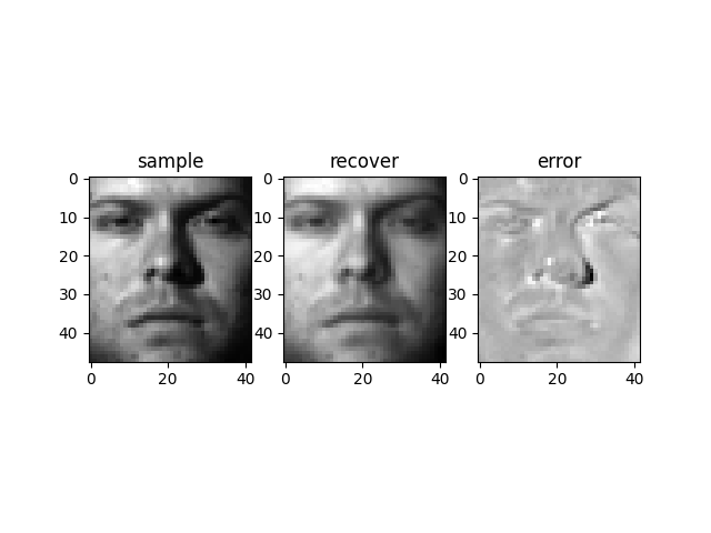
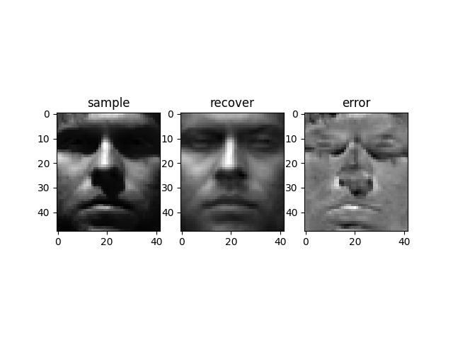
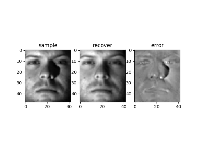
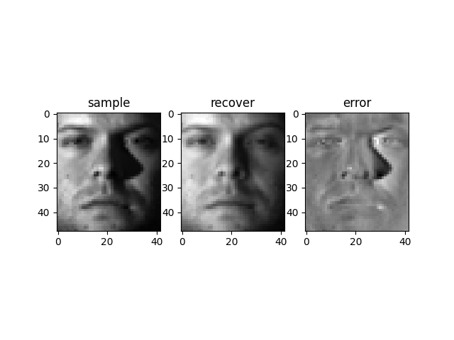
Y 1 ′ = Y 1 + c ∗ ( X − A Z − E ) Y_1' = Y_1 + c*(X-AZ-E) Y 1 ′ = Y 1 + c ∗ ( X − A Z − E ) Y 2 ′ = Y 2 + c ∗ ( Z − J ) Y_2' = Y_2 + c*(Z-J) Y 2 ′ = Y 2 + c ∗ ( Z − J ) Suppose we have m images of n people (n< m), some of
which are heavily corrupted. Want to recover these
images by low-rank representation.
In this example, we use the dataset itself as the
dictionary (i.e. A = X A=X A = X
min . ∣ ∣ Z ∣ ∣ ∗ + λ ∣ ∣ E ∣ ∣ 2 , 1 \text{min}. ||Z||_* + \lambda ||E||_{2,1} min . ∣ ∣ Z ∣ ∣ ∗ + λ ∣ ∣ E ∣ ∣ 2 , 1 s.t. X = X Z + E \text{s.t.} ~~~X = XZ + E s.t. X = X Z + E Here are some results