Locally Weight Linear Regression

Recap

LR: Fit $θ$ to minimize $\sum_{i=1}^m(y^{(i)}-θ^Tx^{(i)})^2$.

LWLR: To evaluate $h_θ(x)$ at a certain $x$, fit $θ$ minimize $\sum_{i=1}^mw^{(i)}(y^{(i)}-θ^Tx^{(i)})^2$,where $w^{(i)} = exp(-\frac{(x^{(i)}-x)^2}{2\tau^2})$.

$\tau$ is the bandwidth parameter, controls how fast weight change with distance $|x^{(i)}-x|$; make $\tau$ fixed, when $|x^{(i)}-x|$ is small, the weight is closed to 1, and closed to 0 when $|x^{(i)}-x|$ is large.

When all $w^{(i)}$'s are equal to 1, then all examples has the same weight 1, that's exactly basic Linear Regression.

(a)

Consider a linear regression problem in which we want to "weight" different training examples differently. Specifically, suppose we want to minimize

(i)

Show that $J(θ)$ can also be written

for an appropiate diagonal $W$, and state clearly what $W$ is.

Since $W$ is a diagonal matrix

So

(ii)

If all the $w^{(i)}$'s equal 1, then the normal equation is

and that the value of $θ$ that minimize $J(θ)$ is given by $(XTX)^{-1}X^T\vec y$. By finding the derivative $∇_θJ(θ)$ and setting that to zero, generalize the normal equation to this weighted setting, and give the new value of $θ$ that minimizes $J(θ)$ in closed form as a function of $X$, $W$ and $\vec y$.

Linear Algebra Lemma:$∇_xX^TAX = 2X^TA$

When all $w^{(i)}$'s equal 1

$θ$ is same just the normal linear regression.

(iii)

Suppose we have a training set $\{(x^{(i)},y^{(i)});i=1,2,...,m\}$ of m independent examples, but in which the $y^{(i)}$'s were observed with differing variances.Specifically, suppose that

I.e. $y^{(i)}$ has mean $θ^Tx^{(i)}$ and variance $(\sigma^{(i)})^2$(where the $\sigma^{(i)}$'s are fixed constants). Show that finding the maximum likelihood estimate of $θ$ reduces to solving a locally weighted linear regression. State clearly what the $w^{(i)}$ are in terms of the $\sigma^{(i)}$'s.

Since $\sigma^{(i)}$'s fixed, maximizing $l(θ)$ is equvilent to minimizing

this equation is in the form of locally weighted linear regression, where $w^{(i)} = \frac{1}{2(\sigma^{(i)})^2}$.

So fixing a Gaussian Distribution is somehow like fixing a LWLR?

(b)

Training dataset is provided here and testing data is provided here

(i)

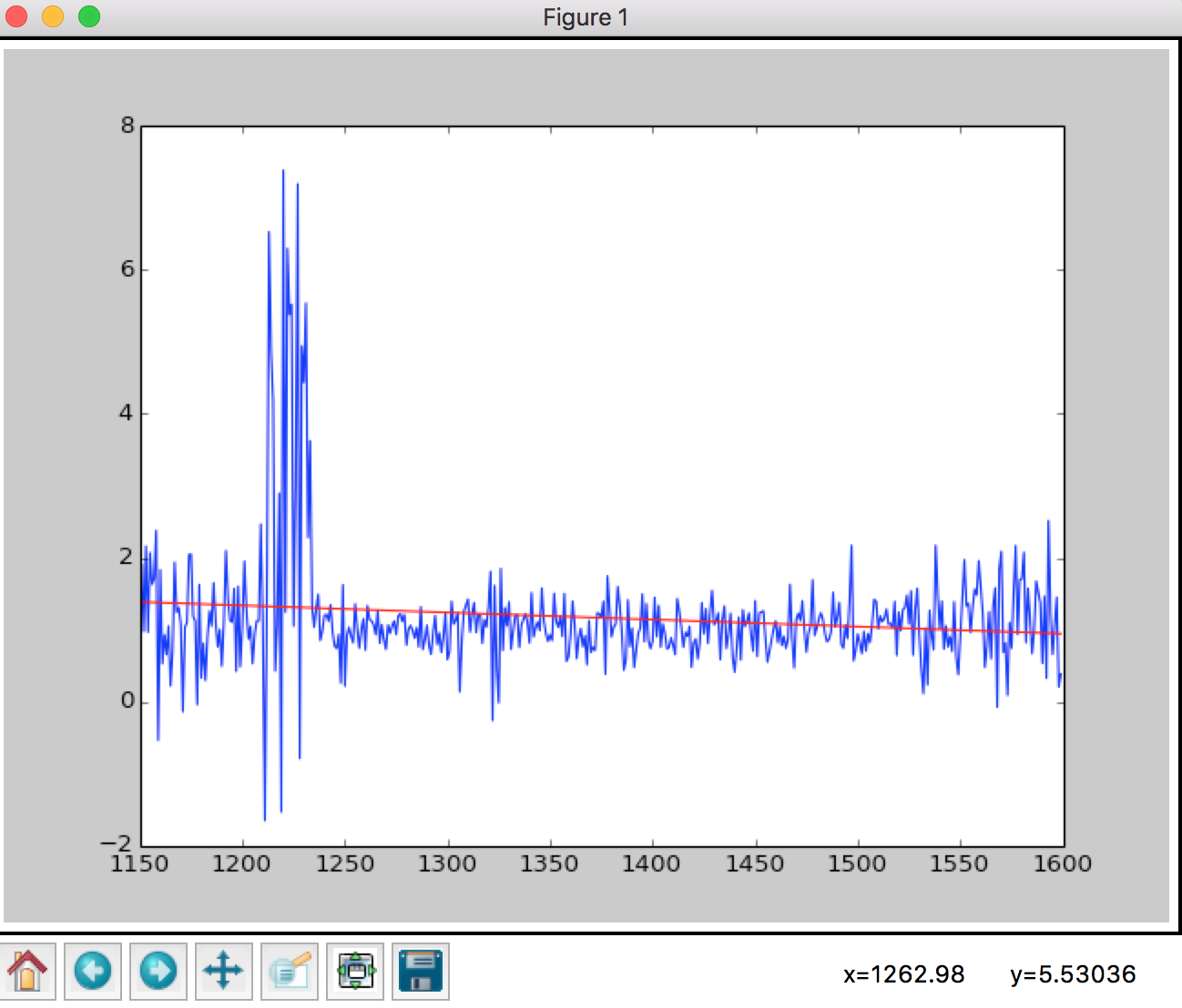
Use the normal equations to implement (unweight) linear regression on the first training example. On one figure plot both the raw data abd tge straight line resulting from your fit. State the optimal $θ$ resulting from linear regression.

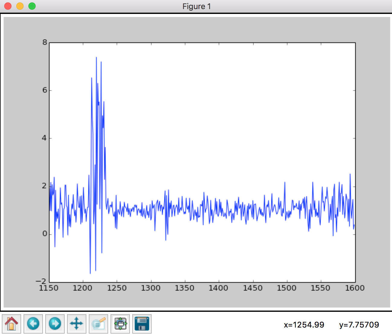
First let plot the raw data.

import pandas as pd
import matplotlib.pyplot as plt

quasar_train = pd.read_csv("quasar_train.csv")
wave_lengthes = quasar_train.columns.values.astype(float).astype(int)

plt.plot(wave_lengthes, quasar_train.values[0])

Now let do the math stuff.

First, a function to get local weights. For a single x, have a serial of weights respect to diffent distance.

And again, here's the $θ$ formula.

When $w^{(i)}$'s equal 1, then it's same as linear regression.

import numpy as np

def getLocalTheta(X, Y_vector, Weight_mat = None):
        if Weight_mat is None:
        return np.linalg.inv(X.T.dot(X)).dot(X.T).dot(Y_vector)
    else:
        return np.linalg.inv(X.T.dot(Weight_mat).dot(X)).dot(X.T).dot(Weight_mat).dot(Y_vector)
        

X1 = np.ones(shape=[len(wave_lengthes)])
X = np.stack([wave_lengthes, X1]).T

theta = getWeightedTheta(X, quasar_train.values[0],None)

plt.plot(wave_lengthes, quasar_train.values[0])
plt.plot(wave_lengthes, X.dot(theta),'r')
plt.show()

Looks like this

(ii)

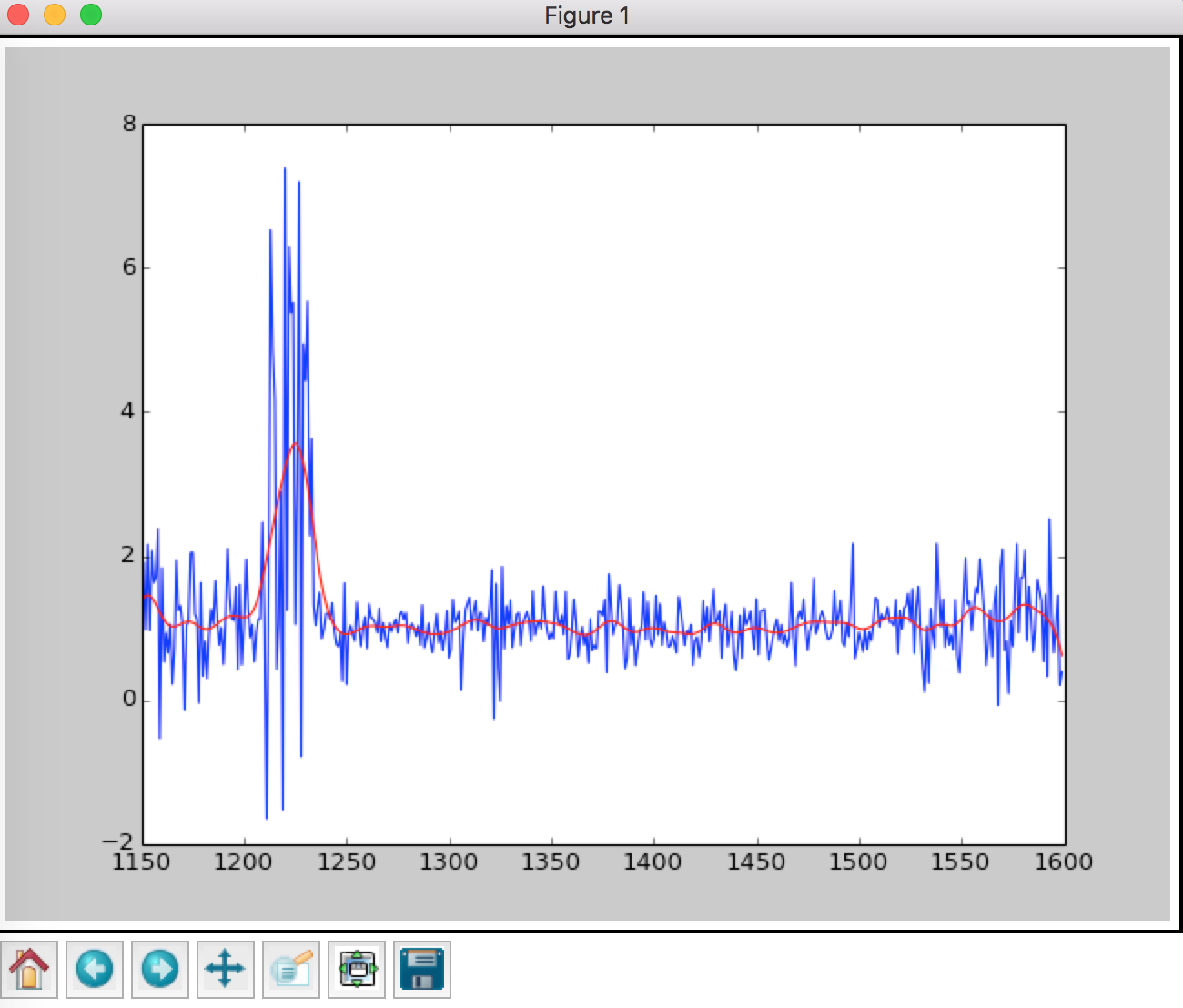
Implement locally weighted linear regression on the first training example. Use normal equations you derived. When evaluating $h()$ at a query point x,use weights

with bandwidth parameter $\tau=5$.

def getLocalWeights(x, X_range, Tau):
    return np.diag(
        np.exp(
            (-(x-X_range[:])**2)/(2 * Tau**2)
        )
    )
    
def getWeightedRegression(X_range, Y_vector, tau):
    X1 = np.ones(shape=[len(X_range)])
    X = np.stack([X_range,X1]).T
    Weighted_Y = []

    for x in X:
        localWeights = getLocalWeights(x[0], X_range, tau)
        localTheta = getWeightedTheta(X, Y_vector, Weight_mat=localWeights)
        Weighted_Y.append(x.dot(localTheta))

    return Weighted_Y
    
first_example = quasar_train.values[0]
weighted_wave = getWeightedRegression(wave_lengthes, first_example,5)

plt.plot(wave_lengthes, first_example,'b')
plt.plot(wave_lengthes, weighted_wave,'r')
plt.show()

For each query point x we perform weighted linear regression, notice that when getting weighted theta, we use uppercase $X$.

And the weighted regression looks like

For sake of layout, we place

def getLocalWeights(x, X_range, Tau):
def getWeightedTheta(X, Y_vector, Weight_mat = None):
def getWeightedRegression(X_range, Y_vector, tau):

into functions.py

(iii)

Repeat (b)(ii) four more times with $\tau =1,10,100$ and $1000$, plot the resulting curves. In 2-3 sentences comments on what happens to the locally weighted linear regression line as $\tau$ varies.

import functions as fn
import pandas as pd
import matplotlib.pyplot as plt

qusar_train = pd.read_csv('quasar_train.csv')
first_example = qusar_train.values[0]
wave_lengthes = qusar_train.columns.values.astype(float).astype(int)

fig, axes = plt.subplots(2,2)
axes = axes.ravel()
for k,tau in enumerate([1,10,100,1000]):
    ax = axes[k]
    weightedWave = fn.getWeightedRegression(wave_lengthes, first_example, tau)
    ax.plot(wave_lengthes, first_example, 'r')
    ax.plot(wave_lengthes, weightedWave, 'b')
    ax.set_title('Tau={}'.format(tau))

plt.legend(loc='best')
plt.show()

And looks like this

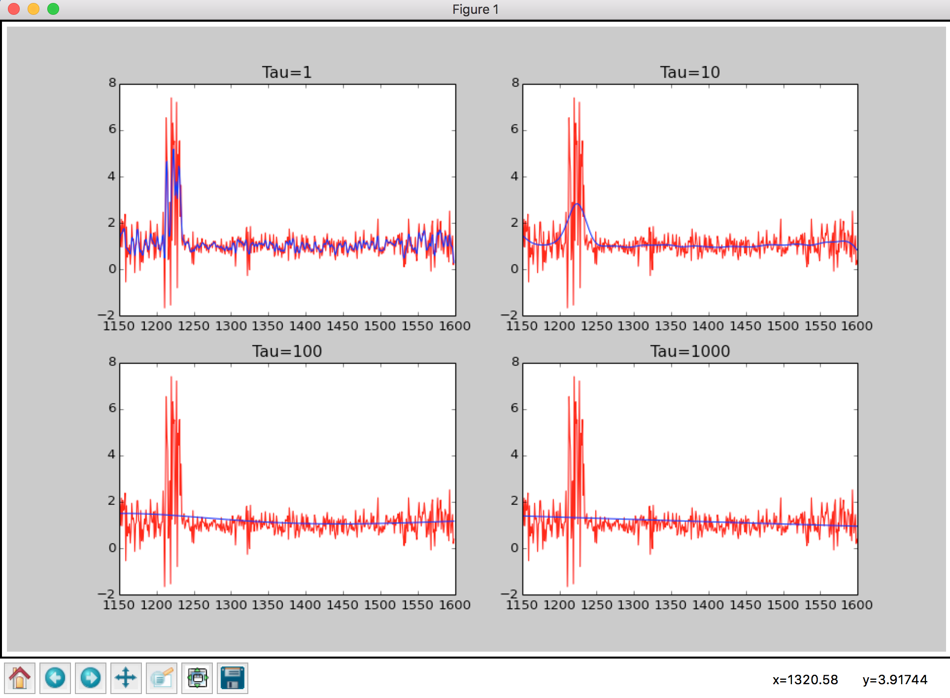
Namely, $\tau$ is the bandwidth parameter, from the formula

we can see that, when the distance $|x-x^{(i)}|$ changes, $\tau$ controls how fast $w^{(i)}$ changes, when $\tau$ is very large, the weight barely changes, so the line is more smooth.