Definition

Orthogonality

Which means $cosmt$ forms a set of orthogonal functions on the interval $[-1,1]$.

Let $t=arccos(x)$,$t∈[0,\pi]$, then $x=cost$, $x∈[-1,1]$

Since the Chebyshev Polynomial gives a set of orthogonal functions on the interval $[-1,1]$, any continuous, real-valued funcion$f(x)$ can be expanded as a series of Chebyshev Polynomials.

Like Fourier Series, to compute $A_k$, we "mask out" other terms in the series.

And to convert it back to Fourier-like projection, let $t=arccos(x)$,$x∈[-1,1]$, then $x=cos(t)$,$t∈[0,\pi]$.

Zeros of $T_n(x)$

Discrete Chebyshev Expansion

Chebyshev Polynomials has the discrete orthogonality property

where $N > m,n$ and $x_k$ is the zeros of $T_N(x)$

TODO: since $f_N(x_k)$ in terpolates $f$ at $N+1$ chebyshev nodes

write $f(x_k)$ as chebyshev expansion

so we have

To get $A_0$, set $m=0$, all $T_n(x_k) T_m(x_k)$ is $0$ except $T_n(x_k) T_m(x_k)=N$ when $m=n=0$

To get $A_j~(j!=0)$, set $m=j$, all $T_m(x_k) T_n(x_k)$ is $0$ except $T_m(x_k) T_n(x_k) = \frac{N}{2}$ when $m=n!=0$

where $x_k = cos( \frac {2k-1} {2N}\pi )$ since the approximation is null only at these points. TODO: why

Approximate A function with Chebyshev

In the previous sections, we reached the conclusion that any function can by written as expansion of chebyshev polynomial.

Furthermore, the chebyshev basis can be calculated recursively and the chebyshev coefficients can by calculated with summation instead of integral.

If we approximate a function with $K$-order chebyshev polynomial, the chebyshev coefficients are given by

where $j$ goes from $0$ up to $K$, and $x_k = cos( \frac {2k-1} {2N} \pi )$ where $N>j$

Typically we just choose $N = K+1$,and the approximated function is $f(x) = \sum_{i=0}^K A_i(x)T_i(x)$

So, first we need a function to compute the chebyshev basis which is done recursively according to the recursive relation of chebyshev polynomial

import numpy as np
K = 6
def chebyshev_basis(K, xs):
    """ Compute the chebyshev basis from T_0(xs) up to T_{K-1}(xs) """
    T = np.zeros(shape=(K, xs.size))
    T[:,0] = np.ones_like(xs)
    T[:,1] = xs
    for k in range(2,K):
        T[:,k] = 2 * xs * T[:,k-1] - T[:,k-2]
    return T
    
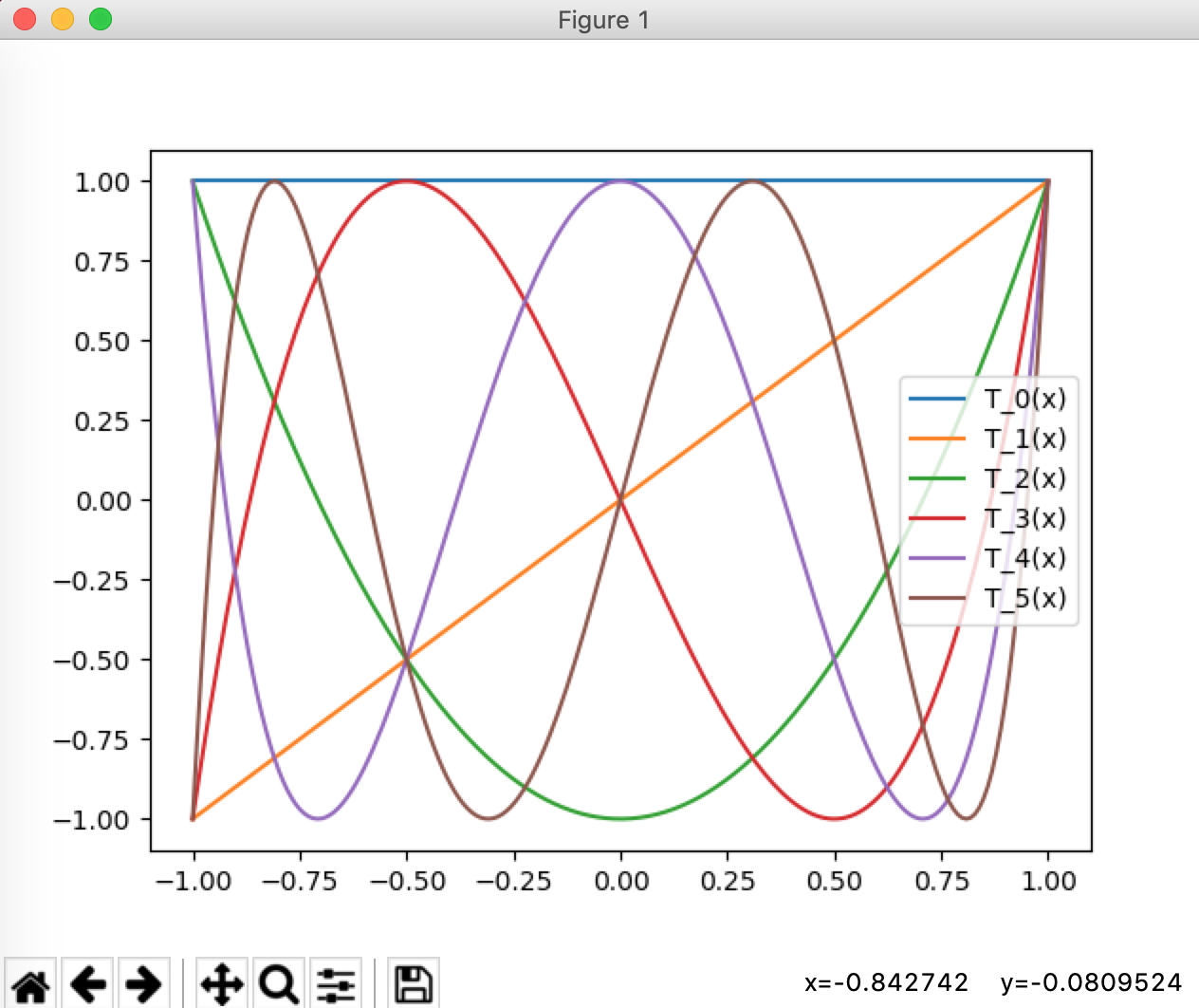
xs = np.linspace(-1,1,200)  # remember that the domain of T_m(x) is [-1,1]
T = chebyshev_basis(K, xs)
for i in range(K):
    plt.plot(xs, T[:,i], label="T_{}(x)".format(i))
plt.legend(loc='best')
plt.show()

The chebyshev basis looks like

Then we need a function to compute the chebyshev nodes

def chebyshev_nodes(K):
    """ Compute the zeros of T_k(x) """
    return np.cos(
        np.pi * (np.arange(K) - 0.5) / K
    )

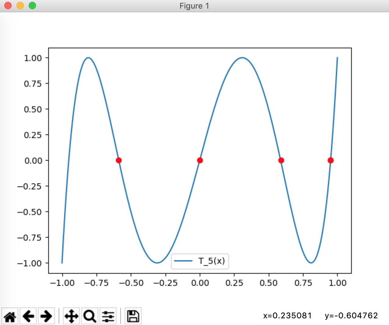
xs = np.linspace(-1,1,200)  # remember that the domain of T_m(x) is [-1,1]
T = chebyshev_basis(K, xs)
nodes = chebyshev_nodes(K-1)

plt.plot(xs, T[:,K-1], label="T_{}(x)".format(K-1))
plt.plot(nodes, np.zeros_like(nodes), 'ro')
plt.legend(loc='best')
plt.show()

$T_k(x)=0$ at chebyshev nodes, that what we expected.

Finally we need a function to compute chebyshev coefficients

def chebyshev_coefficient(K, f):
    """
    Compute the chebyshev coefficients from A_0 up to A_{K-1}
    using chebyshev nodes of T_K(x)
    """
    nodes = chebyshev_nodes(K)
    basis = chebyshev_basis(K, nodes)
    c = np.zeros(K)

    for k in range(K):
        c[k] = 2 / K * np.sum(f(nodes) * basis[:,k])
    c[0] /= 2
    return c

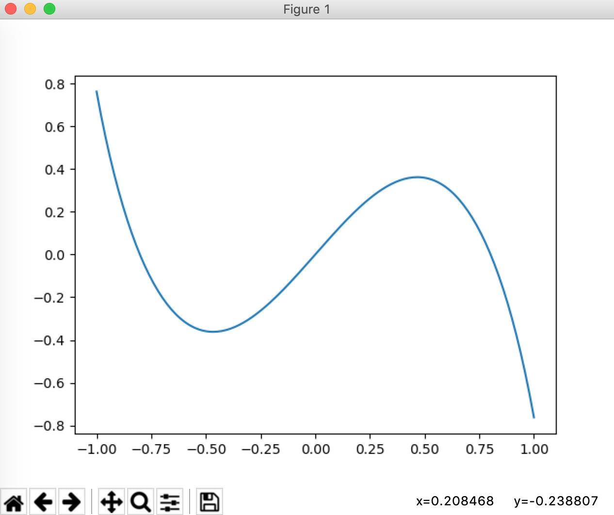
To test the chebyshev approximation, first we construct a fairly complicated function

xs = np.linspace(-1,1,200)  # remember that the domain of T_m(x) is [-1,1]
f = lambda x : np.sin(2*x) - 0.92 * np.tan(1.1 * x)  + 0.18 * np.tanh(0.98 * x)
plt.plot(xs, f(xs))
plt.show()

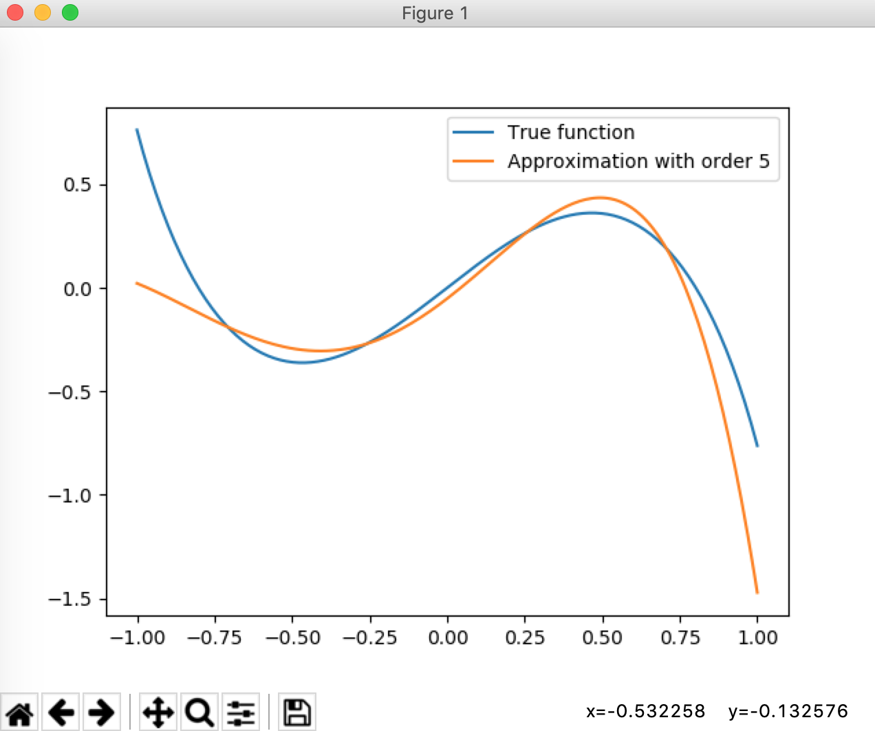
Then we compute the chebyshev coefficients and chebyshev basis and reconstruct the function.

xs = np.linspace(-1,1,200)  # remember that the domain of T_m(x) is [-1,1]
f = lambda x : np.sin(2*x) - 0.92 * np.tan(1.1 * x)  + 0.18 * np.tanh(0.98 * x)

c = chebyshev_coefficient(K, f)
# remeber when we pass the parameter K, actually we get basis up to order K-1
basis = chebyshev_basis(K, xs)

ys = np.zeros_like(xs)
for k in range(K):
    ys += c[k] * basis[:,k]

plt.plot(xs, f(xs), label='True function')
plt.plot(xs, ys, label='Approximation')
plt.show()

And try different $K$